Affiliate links help support this site at no extra cost to you.
The $3 AI Chip: How to Run TinyML on ESP8266 (No Cloud Required)
Artificial Intelligence is usually associated with massive data centers, burning kilowatts of power, and costing thousands of dollars per hour.
But what if I told you that you can run a Neural Network on a chip that costs less than a cup of coffee?
And what if I told you it could run on a coin cell battery for months?
Welcome to TinyML.
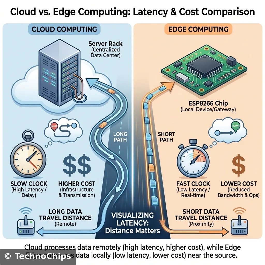
This is the frontier of “Edge Computing”. Instead of sending data to the Cloud (slow, insecure, expensive), we process it locally on the silicon.
Today, we will turn your humble ESP8266 into a brain capable of recognizing gestures, words, or anomalies.
The Problem: The “Cloud” Disconnect
Why do we need TinyML?
Latency: If a self-driving car sees a pedestrian, it cannot wait 200ms to ask a server what to do. It must decide now.
Bandwidth: Streaming raw accelerometer data 24/7 consumes GBs of data. Sending a single byte (“Anomaly Detected”) consumes nothing.
Privacy: Smart speakers that listen to everything you say are creepy. A chip that only wakes up when it hears a keyword (locally) is safe.
Power: Wi-Fi radios are power-hungry (100mA+). A CPU crunching math is efficient (10mA).
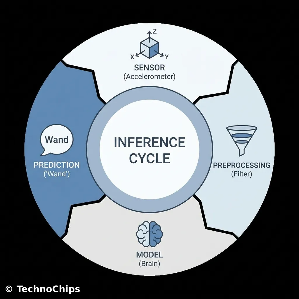
How it Works: The TinyML Pipeline
You cannot train a model on an ESP8266. It lacks the RAM (50kb vs 16GB).
Instead, we use a pipeline:
Capture Data: Use the ESP8266 to record raw sensor data (e.g., “Waving Wand”).
Train Model: Upload data to a powerful machine (Google Colab) to learn the patterns.
Convert: Squash the massive model into a tiny “Lite” version (Quantization).
Deploy: Upload the C++ Byte Array back to the ESP8266.
Inference: The ESP8266 runs the math in real-time.
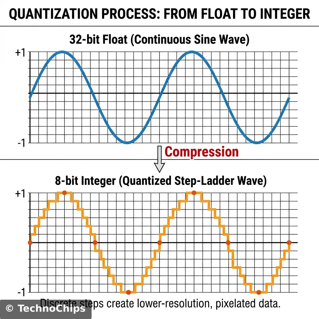
Technical Deep Dive: Quantization (Int8 vs Float32)
Standard Neural Networks use 32-bit Floating Point numbers (e.g., 0.156294).
Problem: Floats are slow to calculate on simple CPUs and take up 4 bytes each.
Solution:Quantization. We map all those complex decimals into 8-bit Integers (-128 to 127).
Real_Value=(Integer−Zero_Point)×Scale
Result: The model shrinks by 4x. The accuracy drop? Usually less than 1%.
This is how we fit a brain into 50kb of RAM.
Step 1: Data Collection (The Gesture)
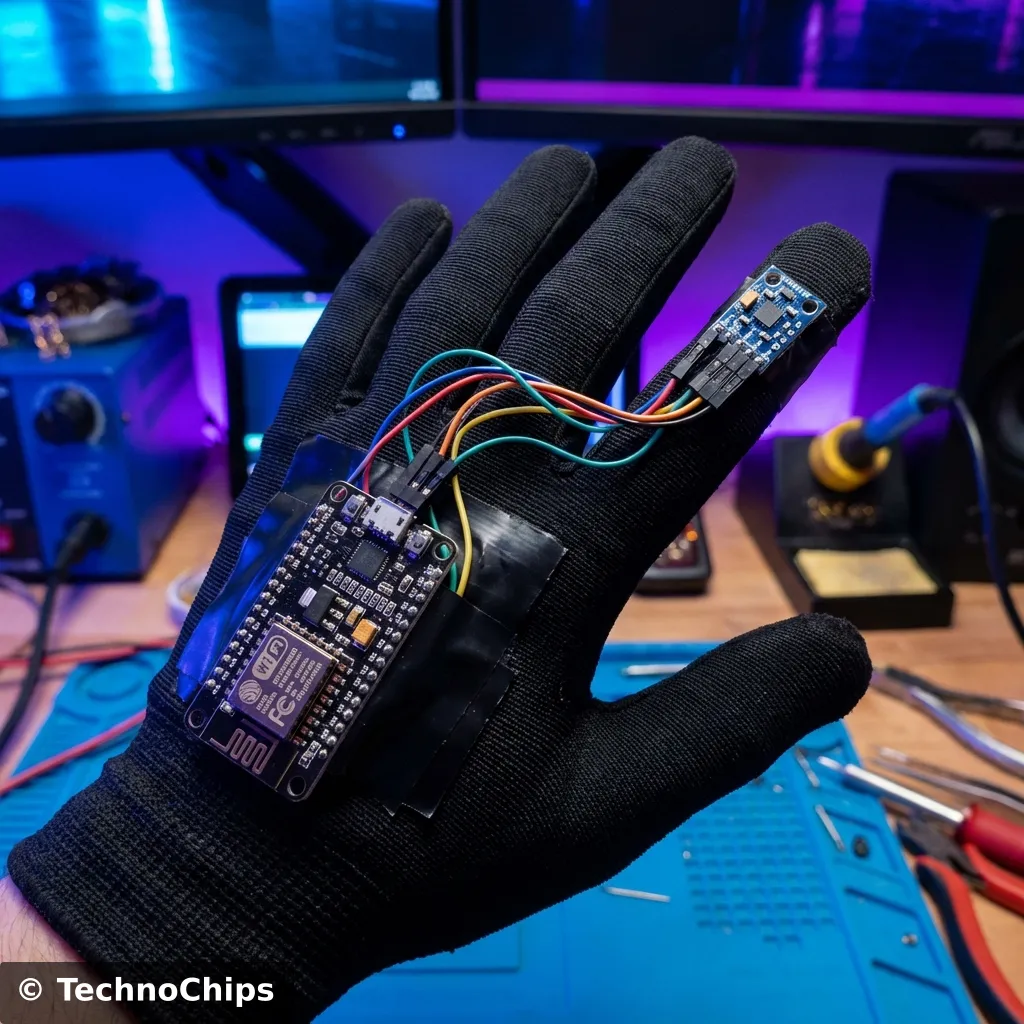
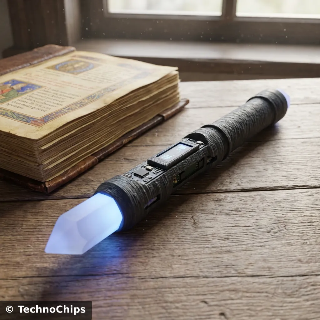
We will build a “Magic Wand”.
Hardware: ESP8266 + MPU6050 (Accelerometer).
Goal: Recognize “W” (Wingardium Leviosa) vs “Circle” vs “Strike”.
The Code (Data Logger):
We need to sample the accelerometer at exactly 100Hz and print it to Serial.
#include <Adafruit_MPU6050.h>#include <Adafruit_Sensor.h>#include <Wire.h>Adafruit_MPU6050 mpu;void setup() { Serial.begin(115200); if (!mpu.begin()) { while (1) yield(); } mpu.setAccelerometerRange(MPU6050_RANGE_8_G); mpu.setGyroRange(MPU6050_RANGE_500_DEG); mpu.setFilterBandwidth(MPU6050_BAND_21_HZ);}void loop() { sensors_event_t a, g, temp; mpu.getEvent(&a, &g, &temp); // Print raw data for Python to grab Serial.print("DATA,"); Serial.print(a.acceleration.x, 3); Serial.print(","); Serial.print(a.acceleration.y, 3); Serial.print(","); Serial.print(a.acceleration.z, 3); Serial.println(); delay(10); // Approx 100Hz}
1.1 The Code Explained: Why 100Hz?
You might notice delay(10). Neural Networks need consistent timing.
If you train your model on data sampled at 50Hz, but your wand runs at 100Hz, the gesture will look “slow motion” to the brain. It will fail.
The Serial Format: We print DATA,x,y,z.
The Baud Rate:115200. Do not use 9600. Sending floats takes time. If the print takes 20ms, you can’t sample at 10ms (100Hz).
The Range:MPU6050_RANGE_8_G. A wand wave is violent. 2G is too easily maxed out (clipping). 8G gives us headroom.
Step 2: Training in Google Colab
We don’t have a GPU. Google does. And they let us use it for free.
We use TensorFlow Lite for Microcontrollers.
Key Python Concepts:
Windowing: We chop the continuous stream of motion into 2-second “Windows”.
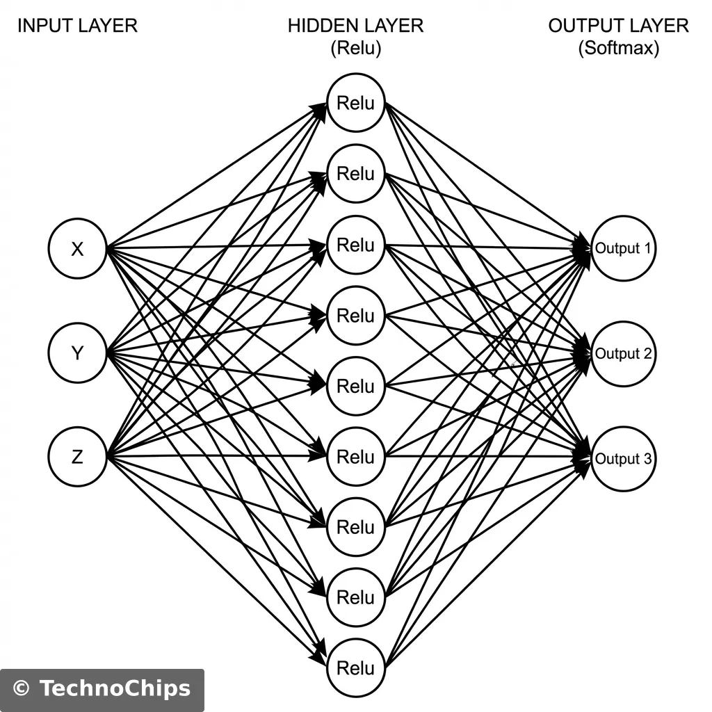
CNN (Convolutional Neural Network): Yes, CNNs are for images, but a time-series graph is an image (Time x Axis).
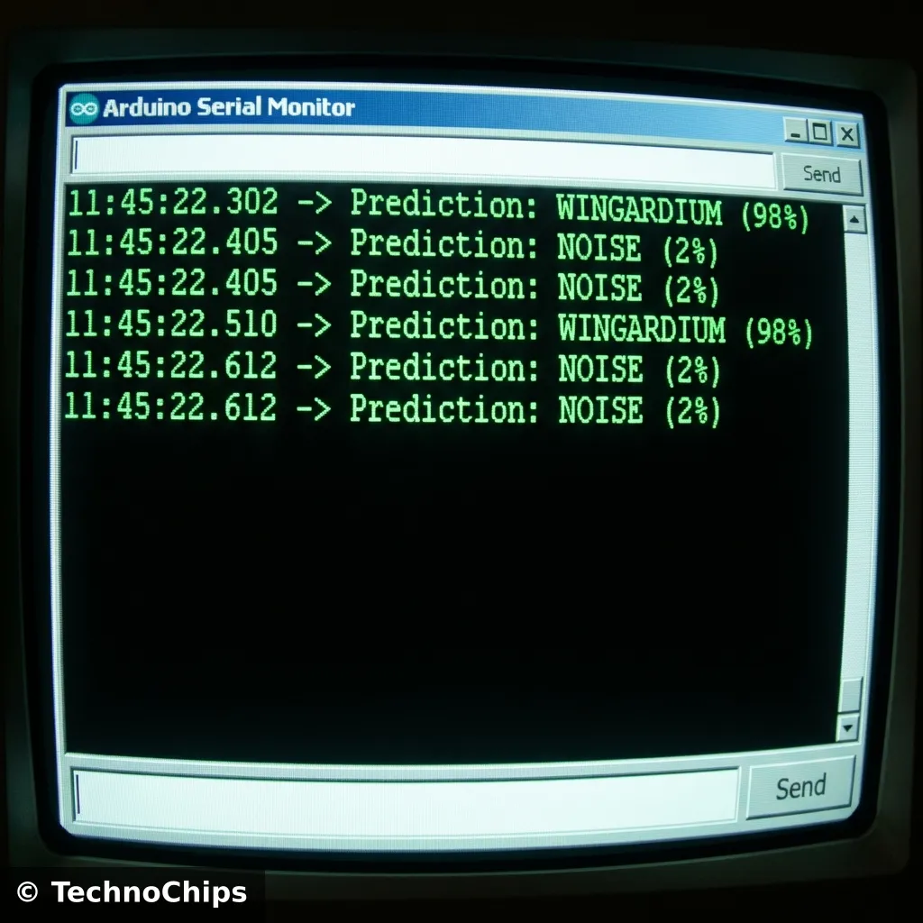
Softmax: The output layer gives probabilities that sum to 1.0 (e.g., [Wingardium: 0.9, Noise: 0.1]).
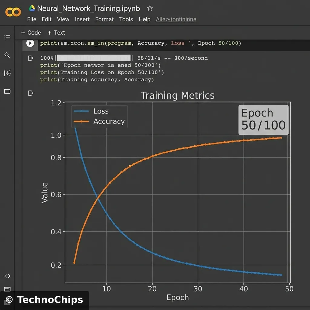
The Training Graph:
Watch the “Loss” curve. It should plummet like a stone. If it oscillates, your learning rate is too high.
Watch the “Validation Accuracy”. If Training Accuracy >> Validation Accuracy, you are Overfitting (memorizing the test questions).
Step 3: The Conversion (xxd)
Once trained, we export a .tflite file.
But the ESP8266 IDE doesn’t know what a file is. It knows C++.
We run a command (on Linux/Mac):
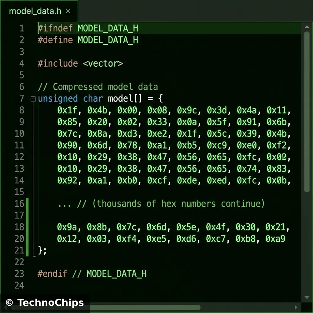
xxd -i gesture_model.tflite > model.h
The Output:
A massive C array. This is your frozen brain.
You might wonder why we don’t just load the .tflite file from SPIFFS.
We could, but converting it to a C array allows the compiler to store it in PROGMEM (Flash Memory) easily.
The format isn’t random. It uses FlatBuffers.
Zero-Copy: The library doesn’t need to parse or unpack the model. It just points to memory addresses inside this array.
Memory Efficiency: This is critical for microcontrollers. A JSON or XML model would require parsing (spending RAM). FlatBuffers are ready-to-eat.
Technical Deep Dive: The TensorFlow Lite Micro Architecture
How does Google fit TensorFlow into 50KB?
No Dynamic Memory:malloc() is banned. Everything is allocated upfront in the “Tensor Arena”.
Operator Kernels: Standard TensorFlow has thousands of ops (Conv2D, LSTM, Softmax). TFLite Micro only includes the specific handful of “Micro Mutable” ops you actually use.
Static Graph: The execution plan is baked in. No changing the network shape at runtime.
Variable Quantization
We talked about int8. But not all int8s are equal.
Symmetric Quantization: simple mapping centered around 0.
Asymmetric Quantization: Uses a “Zero Point” offset. Better for ReLu layers (which are 0 to infinity).
Per-Channel Quantization: Different scaling factors for each filter in a Convolution layer.
Why care? If your model accuracy sucks after conversion, switch from Asymmetric to Symmetric.
Step 4: Inference Engine (The ESP8266 Code)
This is the hardest part. Wiring TensorFlow into the Arduino environment.
We use the TensorFlowLite_ESP32 library (it works on 8266 mostly, or use EloquentTinyML wrapper for sanity).
The Interpreter:
Think of the Interpreter as the “Player” for your model file.
Allocate Arena: We reserve a chunk of RAM (e.g. 10kb) for the math scratchpad.
Set Input: We feed our live accelerometer buffer into input->data.f.
Architectural Considerations: Why not Raspberry Pi?
You might ask, “Why suffer with 50kb RAM? Just use a Pi Zero.”
Boot Time: Pi takes 30s to boot Linux. ESP8266 takes 200ms.
Integrity: You can pull the plug on an ESP8266. Do that to a Pi and you corrupt the SD card.
Hard Real-Time: Linux can pause your code to update system logs. Microcontrollers do exactly what you say, when you say it.
Common Pitfalls (The “Gotchas”)
1. The “Ghost” Inputs
Neural Networks are excellent interpolators but terrible extrapolators.
If you train it on “Wave” and “Punch”, and then you do a “Clap”, it won’t say “Unknown”. It will say “Wave (51%)”.
Fix: You must train a “Background Class” or “Noise Class” containing random movements.
2. Memory Fragmentation
The Tensor Arena must be a contiguous block of RAM. If you use String objects or heavy heap allocation elsewhere, you might fragment the RAM so much that the Arena can’t fit, even if total free RAM is high.
Fix: Allocate the Arena globally and static.
3. Sampling Jitter
If your training data was sampled at 99Hz, 101Hz, 100Hz… but your inference loop runs at exactly 100Hz, the shapes will be warped.
Fix: Use micros() to enforce strict timing loops.
Optimization Techniques: Squeezing the Lemon
Your model is too big? Too slow?
Pruning: Remove connections (weights) that are near zero. A “sparse” brain works just as well.
Depthwise Separable Convolutions: Standard Conv2D is expensive (N×N×Channels). Depthwise splits this into two cheaper operations. This is how “MobileNet” works.
Clock Speed: The ESP8266 runs at 80MHz by default.
system_update_cpu_freq(160);
This doubles your inference speed instantly (at the cost of heat).
The “Hello World” of AI: Sine Wave Approximation
Before you build the wand, try to predict a Sine Wave.
Input:x (Time).
Output:y=sin(x).
Why? It proves your toolchain works without worrying about messy sensors. If your chip can’t predict a curve, it can’t predict a wand_wave.
Troubleshooting TinyML: When the Brain Fails
Deploying AI to a $3 chip is not seamless. Here is how to fix the common crashes.
1. The “Arena Exhausted” Panic
The most common error is TensorArena allocates X bytes but needs Y.
Cause: Your model is too fat, or your TENSOR_ARENA_SIZE is too small.
Fix: Increase the size in 1kb increments. If you hit the ESP8266 RAM limit (roughly 40kb usable for heap), you must simplify the model (fewer layers, fewer neurons).
2. The Shape Mismatch
Training says: Input shape: [1, 60].
Inference says: Invoke() failed.
Cause: You are feeding 59 floats or 61 floats.
The Math: 100Hz sampling for 2 seconds = 200 samples. 3 Axes (X,Y,Z). 200×3=600 inputs.
The Fix: Hardcode the buffer size using #define. Never use dynamic vector.push_back.
3. The Endianness Trap
You trained on x86 (Intel, Little Endian). You deploy to a microcontroller (Usually Little Endian, but some are Big Endian).
TFLite Micro handles this: Mostly. But if you manually bit-bang weights, you will get garbage predictions. Always use the standard xxd or Python conversion scripts.
Frequently Asked Questions (TinyML Edition)
Q: Can I do Voice Recognition on ESP8266?
A: Barely. The “Micro Speech” demo requires a PDM microphone and heavy DSP (Fast Fourier Transform). The ESP8266 is a bit underpowered for real-time audio. Use an ESP32 (dual core) for “Ok Google” style keywords.
Q: How does this affect Battery Life?
A: AI is expensive. Running the CPU at 160MHz drains the battery in hours.
Strategy: Keep the ESP8266 in Deep Sleep. Use an external ultra-low-power accelerometer (like ADXL345) to detect “motion”. Only WAKE the ESP8266 when motion is detected to run the Inference.
Q: My model works in Colab but fails on the Chip!
A: This is usually “Data Drift”. Your training data came from a clean dataset. Your real-world data is noisy.
Solution: Collect “Validation Data” using the chip itself. Record yourself waving the wand and add THAT to the training set.
Final Project: The “Smart Wand”
Imagine a Harry Potter wand that actually controls your smart home.
Gestures:
Circle: Turn on Living Room Lights.
Thrust: Lock the Front Door.
Swipe Up: Open Blinds.
Shake: Party Mode (Disco lights).
Hardware:
ESP8266 (WeMos D1 Mini) fits inside a PVC pipe.
MPU6050 Accelerometer taped to the tip.
LiPo Battery (18650) in the handle.
This is not Science Fiction. This is $10 of parts and an afternoon of coding.
You have crossed the threshold from “Programmer” to “AI Engineer”.
Glossary: Speak Like an AI Engineer
Inference: The act of running a model to make a prediction. (Contrast with Training).
Quantization: Reducing the precision of numbers (e.g. 32-bit float to 8-bit integer) to save memory and speed up math.
Tensor: A multi-dimensional array of numbers. A matrix is a 2D tensor.
Tensor Arena: A reserved block of RAM where TFLite Micro stores input, output, and intermediate calculation data.
FlatBuffer: A serialization format by Google that allows accessing data without parsing/unpacking it first.
Epoch: One complete pass through the entire training dataset.
Overfitting: When a model memorizes the training data but fails on new data. (Like memorizing answers to a test).
Loss Function: A math formula that tells the Neural Net how “wrong” it is. The goal of training is to minimize this number.
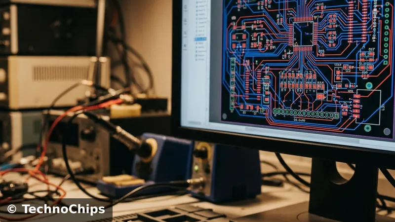
Stop using breadboards. Learn how to design professional Printed Circuit Boards (PCBs) using EasyEDA. A complete step-by-step guide from Schematic to Gerber files for your Smart Home Hub.